There are many operators in RapidMiner. Some are rarely mentioned but deserve to be more widely known because they can do something that would otherwise need a lot of dangerous and exhausting gymnastics (and as a side note, the origin of the word gymnastics comes from a Greek word for naked; you have been warned).
Two such operators are "Fill Data Gaps" and "Replace Missing Values (Series)".
The first of these examines the id attributes of an example set, arranges them in order and works out if there are any missing (integer id attributes are important - using other types causes problems). If there are it will do its best to create new examples to fill the gaps. An illustration is always helpful so imagine you have 5 examples with ids 1,2,5,6,7. The "Fill Data Gaps" operator will create 2 new examples with ids of 3 and 4. Any new examples will be created with all the attributes within the example set but of course these will be set to missing. This is where the second operator can be useful.
The "Replace Missing Values (Series)" operator is part of the series extension so it perhaps doesn't get out as often as it should but it's very useful. Given a load of missing values, it will try and fill them in by assuming the examples form a series. It works on individual attributes in example sets only and treats each attribute as part of a sequential series. As it works its way along a series, if it encounters a missing value it will try and fill it in based on its parameter settings. These settings are "previous value", "next value", "value" and "linear interpolation". For an illustration, imagine you have 7 examples with attribute att1 set to 10,11,?,?,17,19,20. For example, using the "previous value" setting would cause these missing values to be set to 11 and 11. Using "linear interpretation" would set them to 13 and 15.
I find myself using these operators a lot but I keep forgetting the names; hence this post.
Monday 19 December 2011
Saturday 26 November 2011
Counting words in a document: a better way
A much easier way to count words in a document compared to this previous post is to use the word list that is generated by text processing operators.
This example shows this. It uses the "Wordlist to Data" operator and then does some light gymnastics to calculate the sum and count of words to produce the desired results.
This example shows this. It uses the "Wordlist to Data" operator and then does some light gymnastics to calculate the sum and count of words to produce the desired results.
Tuesday 22 November 2011
Normalizing Rows
The "Normalize" operator normalizes each numerical column (called an attribute in RapidMiner's terminology) within an example set to the desired range. Sometimes, you might want to normalize all the numerical values within a row (called an example within an example set in RapidMiner's terminology). I had to do this while understanding how term frequencies are calculated during document vector creation.
A nifty trick is to transpose the example set, normalize and then transpose it back again and the process here shows a very simple example.
This also shows the result of a document processing step which results in term frequencies for comparison. I recently found that RapidMiner performs a cosine normalization when producing term frequencies (it divides by the square root of the sum of the squares of the frequencies within a row which is equivalent to a document) and I wanted to see what differences show up when the sum of the frequencies is used instead (answer: not much with the data I was playing with).
Edit: added RapidMiner equivalent terminology for rows and columns
Tuesday 25 October 2011
Counting words in a document
Here's an example that counts the total number of words in a document followed by the total number of unique words.
It does this by using the "cut document" operator with the following regular expression.
This splits the document into words and each word is returned as a document based on the result of the capturing group; the brackets define the capturing group; everything inside these is returned as a value. The "Documents To Data" operator converts all the documents, one for each word, into examples in an example set. The text field name is set to "word" and this is used in the later operators.
An "Extract Macro" operator obtains the number of examples. This is the same as the count of all words. An aggregation is performed to count words and another "Extract Macro" operator determines the number of unique words from the resulting example set. These macros are reported as log values using the "Provide Macro As Log Value" operators and the log file is converted to an example set using "Log To Data".
Other regular expressions could be used if you want to ignore numbers and inside the "Cut Document" operator it is possible to have other filtering operators such as stemming.
It does this by using the "cut document" operator with the following regular expression.
(\w+)
This splits the document into words and each word is returned as a document based on the result of the capturing group; the brackets define the capturing group; everything inside these is returned as a value. The "Documents To Data" operator converts all the documents, one for each word, into examples in an example set. The text field name is set to "word" and this is used in the later operators.
An "Extract Macro" operator obtains the number of examples. This is the same as the count of all words. An aggregation is performed to count words and another "Extract Macro" operator determines the number of unique words from the resulting example set. These macros are reported as log values using the "Provide Macro As Log Value" operators and the log file is converted to an example set using "Log To Data".
Other regular expressions could be used if you want to ignore numbers and inside the "Cut Document" operator it is possible to have other filtering operators such as stemming.
Wednesday 12 October 2011
Generate Macro bonus features
I was pleased to discover that some of the functions available in the operator "Generate Attributes" are also available in the "Generate Macro" operator.
For example the following functions work.
concat
contains
matches
index
str
upper
lower
escape_html
replace
and I imagine that similar text processing functions will also work.
I tried date_now() and some other date functions and I got a result that looked like an error (actually quite an interesting error). So I assume date functions cannot be used.
Saturday 17 September 2011
Regular expressions: negative look behind
I'm pleased to report after much gymastics that the regular expression feature "regular look behind" works with the "Replace" operator.
So if you have an attribute containing
"mit seit nach bei gegenuber von zu aus"
and you want to replace everything except the word "von" with "bier" then the following regular expression will do it.
replace what - \w+\b(?<!\bvon)
replace by - bier
The result is
"bier bier bier bier bier von bier bier"
Prost! :)
Monday 15 August 2011
Visualizing discrete wavelet transforms: part II
Here is a process that takes the discrete wavelet transform (it happens to be the Daubechies 4 wavelet in this case rather than the Haar but the results are similar) of some fake data and plots the corresponding results. This is different from the maximum overlap discrete wavelet transform from the previous post.
The result looks like this.
 (the z2 attribute is plotted as the colour using log scaling)
The bottom row is the clean signal (with scaling to make it show up), the 2nd row from the bottom is the noisy signal and the third row from the bottom is the result of the discrete wavelet transform. This is only included for completeness since it does not correspond in the original domain to the signal. For an interpretation of this I found the following in the code of the discrete wavelet transform (in file DiscreteWaveletTransformation.java)
In the case of the "normal" DWT the output value series has just one dimension, and these
coefficients are to be interpreted as follows: the first N/2 coefficients are the wavelet
coefficients of scale 1, the following N/4 coefficients of scale 2, the next N/8 of scale
4 etc. (dyadic subsampling of both the time and scale dimension). The last remaining
coefficient is the last scaling coefficient.
So this means the 4th row from the bottom corresponds to the coefficients of scale 1, the 5th row to scale 2 and so on. The coefficients have been replicated as many times as required to match the x scale.
Note that this differs from the view tradionally presented in the literature where the high frequencies are presented at the top. That's an exercise for another day.
The main difference between this and the previous MODWT example is the unpacking of the DWT result. For this I used a Groovy script. This takes 2 example sets as input and copies the correct parts of the first (the DWT result) into the second (the output that will eventually be de-pivoted).
The output example set that is fed into the Groovy script is created using a "Generate Data" operator since I found this to be the easiest way to generate the example set with the right number of rows and columns.
As before, the graphic shows that the algorithm has seen the presence of the low frequency signal at the expected location from x = 5000 and there is perhaps a hint that something has been spotted at x = 100.
The result looks like this.

The bottom row is the clean signal (with scaling to make it show up), the 2nd row from the bottom is the noisy signal and the third row from the bottom is the result of the discrete wavelet transform. This is only included for completeness since it does not correspond in the original domain to the signal. For an interpretation of this I found the following in the code of the discrete wavelet transform (in file DiscreteWaveletTransformation.java)
In the case of the "normal" DWT the output value series has just one dimension, and these
coefficients are to be interpreted as follows: the first N/2 coefficients are the wavelet
coefficients of scale 1, the following N/4 coefficients of scale 2, the next N/8 of scale
4 etc. (dyadic subsampling of both the time and scale dimension). The last remaining
coefficient is the last scaling coefficient.
So this means the 4th row from the bottom corresponds to the coefficients of scale 1, the 5th row to scale 2 and so on. The coefficients have been replicated as many times as required to match the x scale.
Note that this differs from the view tradionally presented in the literature where the high frequencies are presented at the top. That's an exercise for another day.
The main difference between this and the previous MODWT example is the unpacking of the DWT result. For this I used a Groovy script. This takes 2 example sets as input and copies the correct parts of the first (the DWT result) into the second (the output that will eventually be de-pivoted).
The output example set that is fed into the Groovy script is created using a "Generate Data" operator since I found this to be the easiest way to generate the example set with the right number of rows and columns.
As before, the graphic shows that the algorithm has seen the presence of the low frequency signal at the expected location from x = 5000 and there is perhaps a hint that something has been spotted at x = 100.
Thursday 11 August 2011
Visualizing discrete wavelet transforms
RapidMiner can transform data using wavelet transforms within the value series extension. As part of my endeavour to learn about these I made a process that allows visualisation of the results of a MODWT transform. It's intended to show at a glance what the transformation has done to the data.
Amongst others, it uses the "data to series", "series to data" and "de-pivot" operators and of course the "discrete wavelet transform".
The process creates some fake data consisting of 8192 records. A high frequency square wave is located from position 100 to 600 and a lower frequency wave is located from 5000 to 5500. A significant amount of noise is also added to hide the signal.
If you plot the results of the de-pivot operation and use the block plotter, choose x, y and z2 and set the z2 axis to a log scale, you should see something like this.
 The bottom row corresponds to the pure signal (note its amplitude has been scaled to make it show up better), the next row up the noisy signal and all the rows above that correspond to the different output resolutions of the MODWT transform. The top row is the average for all the signals and should be 0 owing to the normalisations performed on the input data. All of this is produced from the MODWT output using the de-pivot operator after a certain amount of joining gymnastics.
The plot shows that the transform has detected a match from the 5000 point for the original signal. The signal from 100 is not so obvious.
The individual outputs from the MODWT operation are also available. Here for example is a plot of the 6th output (i.e. the 8th row in the graphic above).

Compare this with the raw noisy data.

Clearly there is something in the data and the transform is able to isolate this to a certain extent.
My next process will be one to visualise the DWT rather than the MODWT output.
Amongst others, it uses the "data to series", "series to data" and "de-pivot" operators and of course the "discrete wavelet transform".
The process creates some fake data consisting of 8192 records. A high frequency square wave is located from position 100 to 600 and a lower frequency wave is located from 5000 to 5500. A significant amount of noise is also added to hide the signal.
If you plot the results of the de-pivot operation and use the block plotter, choose x, y and z2 and set the z2 axis to a log scale, you should see something like this.

The plot shows that the transform has detected a match from the 5000 point for the original signal. The signal from 100 is not so obvious.
The individual outputs from the MODWT operation are also available. Here for example is a plot of the 6th output (i.e. the 8th row in the graphic above).

Compare this with the raw noisy data.

Clearly there is something in the data and the transform is able to isolate this to a certain extent.
My next process will be one to visualise the DWT rather than the MODWT output.
Sunday 7 August 2011
Finding processes in the repository
I have a lot of processes and it's sometimes hard to remember the name of one containing something useful. A metadata view and search capability of the repository would be very useful.
While that is being invented, here's a process that scans through a repository and determines the name and location of the processes it finds. It also counts the number of operators used to give a sense of how big the process is. The process recursively scans files with extension ".rmp" from a starting folder. Various document operators including "extract information" and "cut documents" using Xpath are used to process the files and extract information from them. The "aggregate" operator is used to count operators.
One day I will make it into a report that can be viewed using RapidAnalytics.
Other data is also extracted and this could be used if desired.
The default location is the default Windows location of the samples processes; change this to the folder where your repository is.
Some gymnastics were required to get the loop files operator to work correctly. This seems to present zero sized directories when iterating so I was forced to use the "branch" operator to eliminate these. Pointing the loop files operator to the C:\ drive usually results in an error that I haven't got to the bottom of yet.
Thursday 21 July 2011
Ignoring many attributes
The "set role" operator has a nice feature that lets you set the role of an attribute to free text.
By setting the role to something like "ignore" subsequent modelling operators will not process the attribute.
Here's an example that creates some fake data with 4 attributes and then sets three of them to be ignored. This causes the clustering operator to perform more poorly because it ignores some of the attributes.
Note that the roles have to be different so in this case they are "ignore01", "ignore02" and "ignore03". If you set them all to "ignore", an error happens.
Note too that the "set additional roles" dialog is a bit fiddly as it loses focus after each character is typed but it does work.
Thursday 7 July 2011
Using regular expressions with the Replace (Dictionary) operator
The "Replace (Dictionary)" operator replaces occurrences of one nominal in one example set with another looked up from another example set.
By default, this replaces a continuous sequence regardless of its position in the nominal.
For example, if an attribute in the main example set contains the value "network" and the dictionary example set contains the value pair "work", "banana", the result of the operation would be "netbanana".
This is fine but if you want to limit to whole words only then you can use the "use regular expressions" parameter in the replace operator. To make this work, you also have to change the text within the dictionary for the nominal to be replaced with "\b" at the beginning and the end. In regular expression speak, this means match a whole word only.
In addition, if the word to be replaced contains reserved characters (from a regular expressions perspective) then "\Q" and "\E" have to be placed around the word.
One way to do this is to use a "generate attributes" operator and create a new attribute in the dictionary example set using the following expression.
The new attribute would then be used in the "from attribute" parameter of the "Replace (Dictionary)" operator. The "to attribute" would be set to the attribute within the example set dictionary that is the replacement value.
By default, this replaces a continuous sequence regardless of its position in the nominal.
For example, if an attribute in the main example set contains the value "network" and the dictionary example set contains the value pair "work", "banana", the result of the operation would be "netbanana".
This is fine but if you want to limit to whole words only then you can use the "use regular expressions" parameter in the replace operator. To make this work, you also have to change the text within the dictionary for the nominal to be replaced with "\b" at the beginning and the end. In regular expression speak, this means match a whole word only.
In addition, if the word to be replaced contains reserved characters (from a regular expressions perspective) then "\Q" and "\E" have to be placed around the word.
One way to do this is to use a "generate attributes" operator and create a new attribute in the dictionary example set using the following expression.
"\\b\\Q"+word+"\\E\\b"In this case, "word" is the attribute containing the word to be replaced. The "\" must be escaped with an additional "\" in order for it all to come out correctly.
The new attribute would then be used in the "from attribute" parameter of the "Replace (Dictionary)" operator. The "to attribute" would be set to the attribute within the example set dictionary that is the replacement value.
Wednesday 6 July 2011
Initial notes about installing RapidAnalytics in the Cloud and locally
Taking advantage of the Amazon EC2 free year long trial, I installed RapidAnalytics in their Cloud on a micro instance running Ubuntu 10.10 with MySQL. Port 8080 needs to be opened in the instance firewall to allow incoming requests to the RapidAnalytics web page.
Installation of the Ubuntu desktop, a VNC server and Java was the time consuming part. Note that installing Java does not work on a micro instance; there is a known error. The workround is to run on a small instance and then install Java in that environment. Having done that, the image can be saved and re-run on a micro instance.
The memory available in the micro instance is insufficient for the default JBoss settings. Reducing this to 512M allows everything to start but after 30 minutes it does not run properly with many timeout like errors.
Sad conclusion: the micro instance is too small - this is a shame since it means free Cloud practice is not possible.
Changing to a small instance allow things to start and after about 5 minutes, RapidAnalytics starts OK and is usable. This costs money - not a lot - but enough for my mean streak to kick in. A medium instance would presumably start more quickly - it would cost a bit more so I didn't try it.
The IP connectivity to allow the server to be found so that a local RapidMiner client can use it is the next step although money is likely to be required to assign an IP address that can be seen on the Internet.
Conclusion: RapidAnalytics will work in the Cloud but some cost conscious people will choose to install and play on local machines.
Installation on a laptop running XP SP3 and SQL Server is also OK as is installation on a 64 bit laptop running Windows 7 enterprise with MySQL. Note that some SQL Server components steal port 8080 necessitating a change to the JBoss port to something like 8081 in the server.xml file contained in the folder rapidAnalytics\rapidanalytics\server\default\deploy\jbossweb.sar.
Next steps will be to find a way to backup a RapidAnalytics installation and restore on a different machine.
Sunday 12 June 2011
Counting clusters: part R
Here's an example process that uses an R script called from RapidMiner to perform clustering and provide a silhouette validity index.
As before, it uses the same artificial data as for the previous examples; namely 1000 data points in three dimensions with 8 clusters.
The script uses the R package "cluster". This contains the algorithm "partitioning around medoids" which the documentation describes as a more robust k-means.
The process iterates over values of k from 2 to 20, passes the data to R for clustering and generation of an average silhouette value. This allows the optimum value for k to be determined. The "correct" answer is 8 but this may not correspond to the best cluster using the validity measure owing to the random number generator which causes the clusters to differ between each run.
Some points to note
- The R script installs the package and this causes a pop up dialog box to appear. Select the mirror from which to download the package. Comment out the "install.packages" line to stop this (or read the R documentation to work out how to test for the presence of the library before attempting the install).
- The R script takes multiple inputs and these appear as R data frames.
- The output from the R script must be a data frame.
- The returned example set contains the validity measure and this is picked up for logging using the "Extract Performance" operator.
- The order of the processes before the script is important to ensure the correct value of k is passed in. This can be done using the "show and alter operator execution order" feature on the process view.
- The operator "Generate Data By User Specification" is used to create an example set to contain the value of k

A value near 1 is what is being looked for and indicates compact, well separated clusters. The "correct" answer is 8 and the result supports this.
Saturday 4 June 2011
Counting clusters: part IV
Here's an example process that uses the operator "Map Clustering on Labels" to match labels to clusters. If the data already has labels, the operator allows the output from a clustering algorithm to be assessed. It compares labels and clusters and determines the best match. From this, the output is a prediction and this can be passed to a performance operator to allow a confusion matrix to be created.
This allows a clustering algorithm to be used for prediction if training examples are available.
This allows a clustering algorithm to be used for prediction if training examples are available.
Tuesday 31 May 2011
Care needed using the Cross Distances operator
The "Cross Distances" operator is used to determine which examples in one set are closest to those in another.
Here's an example correctly showing the first example from the first set at zero distance from the first example in the second set. In other words, these two examples match.
Here's another example that behaves unexpectedly. In this case, the first example in the first set is shown at zero distance from the first example of the second set even though the attribute names and values do not match.
The reason for this is the order of the attributes in the example sets. The attributes are created in different orders and it is this that determines which attribute pairs are compared when calculating distances. You can see this ordering if you go to the meta data view and show the 'Table Index' column. The special attributes are also important.
Normally, most will find that this is not a problem. However, if you import data from two different sources that are supposed to represent the same data but which have columns in different orders, you will find that the "Cross Distances" operator will not behave as expected.
It is possible to work round this by using the "Generate Attributes" operator to recreate attributes in both example sets in the same order.
Saturday 21 May 2011
Worked example using the "Pivot" operator
Here is an example process using the "Pivot" operator that converts this input data
 into this output data.
 In the input data, each row corresponds to a transaction and sub transaction with an attribute value.
In the output data, the number of rows corresponds to the number of unique transactions. All the sub transactions for a transaction are combined. New attributes are created so that the attribute for a given sub transaction can be found by looking at the name. For example, "attribute_subTransaction2" is the attribute in the input data which comes from the "subTransaction2" rows.
This is done by setting the "group attribute" parameter of the "Pivot" operator to "transactionId" and the "index attribute" parameter to "subTransactionId". This causes grouping by "transactionId" and the values of the subTransactionId are used to create the names of the new attributes in the output data.
The "consider weights" check box allows weights to be handled although it's not clear how these would get fed into the operator; a problem for another day.
Edit: If there is a numeric attribute whose role is "weight", setting the check box above allows this to be aggregated within the group. Refer to myexperiment.org for an example.
The "skip constant attributes" check box should be left unchecked. If checked, an attribute that does not vary within the group, is ignored and will not appear in the output data. The observed behaviour seems to be a little different but that's also for another day.
The process also uses the "Generate Data by User Specification" and "Append" operators to make the fake data.
Sunday 8 May 2011
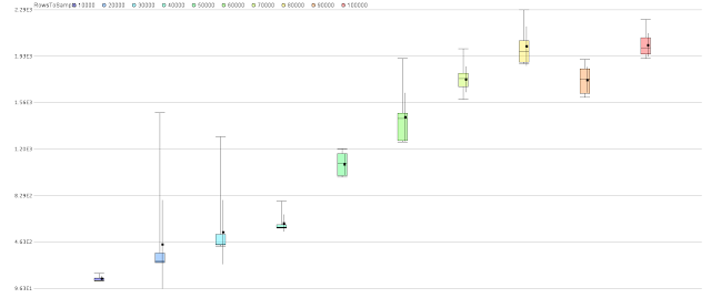
Measuring operator performance for different sizes of data
This process measures the performance of a modelling operator as more and more examples are added. The resultant example set of performance values could be used with a regression model to allow predictions to be made about how a given model will perform with a large data set.
The following values are available for logging with the "Log" operator.
Investigations show that cpu-execution-time and cpu-time are identical and these look like they are measured in microseconds.
Execution-time, looptime and time are also identical to one another and these look like they are measured in milliseconds.
Furthermore, the microsecond values are almost always 1,000 times the millisecond values and therefore, only one of these values is required to allow the measurement to be taken.
The process uses the "Select Subprocess" operator to make it easier to change the model algorithm so avoiding having to edit the "Log" operator. Experiments showed that the timings from the select operator were, to all intents and purposes, identical to those from the enclosed operator.
Performance is not determined solely by the process, there are inevitably external factors that will impact it as other things happen on the computer. The process therefore runs each iteration for a given sample size multiple times to obtain a more statistically meaningful result.
Here is an example quartile colour plot showing performance of a neural network as the number of rows is increased from 10,000 to 100,000 in increments of 10,000.

Here is an example using decision trees.
The following values are available for logging with the "Log" operator.
- cpu-execution-time
- cpu-time
- execution-time
- looptime
- time
Investigations show that cpu-execution-time and cpu-time are identical and these look like they are measured in microseconds.
Execution-time, looptime and time are also identical to one another and these look like they are measured in milliseconds.
Furthermore, the microsecond values are almost always 1,000 times the millisecond values and therefore, only one of these values is required to allow the measurement to be taken.
The process uses the "Select Subprocess" operator to make it easier to change the model algorithm so avoiding having to edit the "Log" operator. Experiments showed that the timings from the select operator were, to all intents and purposes, identical to those from the enclosed operator.
Performance is not determined solely by the process, there are inevitably external factors that will impact it as other things happen on the computer. The process therefore runs each iteration for a given sample size multiple times to obtain a more statistically meaningful result.
Here is an example quartile colour plot showing performance of a neural network as the number of rows is increased from 10,000 to 100,000 in increments of 10,000.

Here is an example using decision trees.

Sunday 1 May 2011
How to read a PMML file to determine the attributes shown on a decision tree
Here is a process to read a PMML file created by RapidMiner.
The PMML file in this case is a model created by running a decision tree algorithm on the iris data set. Here's a snapshot - the highlighted parts are to help explain later.

The result of this XPath is to create multiple documents each containing a small section of the original document. Each section corresponds to the XML for a specific SimplePredicate entry.
Next the process turns the documents into an example set and the number of rows in this corresponds to the number of times the SimplePredicate XPath query cut the file into smaller documents. The example set is returned and after some processing the final output is a list of the attributes used in the decision tree.
In the example, attributes a3 and a4 can be seen on the decision tree and these are also output as an example set.
The PMML file in this case is a model created by running a decision tree algorithm on the iris data set. Here's a snapshot - the highlighted parts are to help explain later.

The process writes this to c:\temp\Iris.xml.pmml and then reads it back in (the subprocess operator allows this to be synchronised). The file is handled as a document by RapidMiner.
Next, the process uses the following XPath to split the document into chunks (the PMML is probably not required).
/xmlns:PMML//xmlns:SimplePredicate
The xmlns is a namespace and this is provided by the following name value pair in the "cut document" operator.
This value is provided in the raw XML and it is important to get this correct. The "assume html" checkbox is unchecked.
The XPath itself simply finds all XML nodes somewhere beneath the PMML node that correspond to "SimplePredicate". By inspection of the PMML, this looked to be the correct way of determining the fields used on the decision tree.
Within the "cut document" operator, the inner operator extracts information using more XPath. This time, the XPath is looking for an attribute named "field" and the XPath to do this is as follows.
A namespace is not required here because it looks like the document fragments don't refer to one.
In the example, attributes a3 and a4 can be seen on the decision tree and these are also output as an example set.
Sunday 10 April 2011
Counting clusters: part III
This process uses agglomerative clustering to create clusters.
As before, the same artificial data as with the k-means and DBScan approaches is used with some of the same cluster validity measures.
The agglomerative clustering operator can create its clusters in three modes. These are single link, average link and complete link. The process iterates over these options in addition to the value of k, the number of clusters.
To extract a cluster from an agglomerative model, the operator "Flatten clustering" must be used.
To make the process more efficient, it would be possible to run the clustering outside the loop operator but that is an exercise for another day. Using the date_now() function within a "Generate attributes" operator would be one way to allow this to be timestamped for those interested in the improvement.
This process also uses the tricky "Pivot" operator. This allows the validity measures for the different modes to be presented as attributes in their own right. To perform this operation, it is necessary to use the "Log to data" operator that turns everything that has been logged into an example set.
Here is an example graph to show how the validity measures vary as k varies. As before, the "correct" answer is 8.

Sunday 3 April 2011
How average within cluster distance is calculated for numeric attributes
The performance for each cluster is calculated first. The cluster density performance operator calculates the average distance between points in a cluster and multiplies this by the number of points minus 1. Euclidean distance is used as the distance measure.
So a cluster containing 1 point would have an average distance of 0 because there no other points.
A cluster containing 2 points would have a density equal to the distance between the points.
Here's a worked example for 3 points. Firstly, here are the points

This table shows the Euclidean distance between them

For example SqrRoot ((-8.625-2.468)^2 + (-5.590-7.267)^2) = 16.981
The average distance of these is 13.726 and the average within distance performance if these three points were in a cluster would be (3-1) times that or 27.452. I'm not quite sure why this multiplication happens (and I have done experiments using 4 points to confirm it and I've looked at the code). I'll leave this comment as a place holder for another day.
Here is what RapidMiner shows.

The negative value is imposed by RapidMiner and seems to be because the best density is the smallest absolute value so negating this means the best density would be the maximum enabling it to be used as a stopping criterion during optimisation.
The performance for all clusters is calculated by summing each cluster performance weighted by the number of points in each and dividing by the number of examples. For example, three clusters with performances -9.066, 0 and -8.943 containing 2, 1 and 3 points respectively would give a result of -7.493 i.e. (2*-9.066+1*0+3*-8.943)/(2+1+3).
What these values mean is a story for another day.
So a cluster containing 1 point would have an average distance of 0 because there no other points.
A cluster containing 2 points would have a density equal to the distance between the points.
Here's a worked example for 3 points. Firstly, here are the points
This table shows the Euclidean distance between them
For example SqrRoot ((-8.625-2.468)^2 + (-5.590-7.267)^2) = 16.981
The average distance of these is 13.726 and the average within distance performance if these three points were in a cluster would be (3-1) times that or 27.452. I'm not quite sure why this multiplication happens (and I have done experiments using 4 points to confirm it and I've looked at the code). I'll leave this comment as a place holder for another day.
Here is what RapidMiner shows.

The negative value is imposed by RapidMiner and seems to be because the best density is the smallest absolute value so negating this means the best density would be the maximum enabling it to be used as a stopping criterion during optimisation.
The performance for all clusters is calculated by summing each cluster performance weighted by the number of points in each and dividing by the number of examples. For example, three clusters with performances -9.066, 0 and -8.943 containing 2, 1 and 3 points respectively would give a result of -7.493 i.e. (2*-9.066+1*0+3*-8.943)/(2+1+3).
What these values mean is a story for another day.
How item distribution performance is calculated for numeric attributes
The item distribution performance operator calculates its performance in the sum of squares case very simply. The number of examples in each cluster is divided by the total number of examples in all clusters. This is squared and the values for each cluster are summed.
For example, three clusters containing 1, 2 and 3 items would have an item distribution score of 0.389. This is 1/36 + 4/36 + 9/36 = 14/36 = 0.389.
For a situation where one cluster dominates and the others clusters are very small in comparison, this value will tend to 1. For the opposite situation, where the clusters have equal numbers of examples, the value tends to 1/N where N is the number of clusters.
Wednesday 30 March 2011
Renaming attributes with regular expressions
If you have an attribute with this name
Firstpart_Secondpart_Thirdpart
and you want to rename it to
Thirdpart_Secondpart_Firstpart
Use the 'Rename By Replacing' operator with this
(.*)_(.*)_(.*)
in the 'replace what' field
and
$3_$2_$1
in the 'replace by' field.
The brackets denote what is known as a capturing group so that everything inside that matches can be used later on by the use of the $1, $2 and $3 entries. The '.*' means match 0 or more characters and will continue until the '_' is found. The capturing group brackets mean that everything from the beginning of the string up to the character before the '_' will be placed into capturing group 1.
Tuesday 22 March 2011
Counting clusters: part II
Here's an example that uses the k-means clustering algorithm to partition example sets into clusters. It uses the same generated data as here but this time it uses different cluster performance operators to determine how well the clustering works.
Specifically there are examples for

Interpreting the shape of these graphs is complex and the subject for another day. In this case, the "right" answer is 8 and the measures don't contradict this.
As usual, the answer does not appear by magic and clustering requires a human to look at the results but the performance measures give a helping hand to focus attention to important areas.
Specifically there are examples for
- Davies-Bouldin
- Average within centroid distance
- Cluster density
- Sum of squares item distribution
- Gini item distribution

Interpreting the shape of these graphs is complex and the subject for another day. In this case, the "right" answer is 8 and the measures don't contradict this.
As usual, the answer does not appear by magic and clustering requires a human to look at the results but the performance measures give a helping hand to focus attention to important areas.
Wednesday 16 March 2011
Discretize by user specification: an example
The Discretize By User Specification operator allows numerical attributes to be placed in bins where the boundaries of the bins are defined by the user. This converts numerical attributes into nominal ones as required by some algorithms.
The following shows some example settings for the operator

The class names show the equality tests. The order of the list is important. The first entry must be the biggest, the last the smallest. Anything lower than the smallest entry is automatically less than "-Infinity". The upper case I on Infinity is important.
These example settings on a small example set are shown below.

The attribute "Copy of att1" is simply a copy of att1 before the discretization.
Tuesday 8 March 2011
Generating reports in a RapidMiner process
Here's an example of a RapidMiner process that generates reports. One report is a PDF, the other is a static Web page.
The basic flow is to start with a "Generate Report" operator. This sets up the name, type and location of the report; in this case a pdf file. From then on, the name of the report is used by subsequent operators to add things to it. In the example, the next operator creates a "series multiple" plot of the attributes of the iris data set plotted against the label. From there, a page break is added and finally another plot is added, this time of the cluster determined from a k-means clustering algorithm. The final report is located in c:\temp\Iris.pdf.
Multiple reports can be created so it would be possible to have many reports created in a single process.
In the example, a "generate portal" operator creates another report and similar graphs are reported to it. In this case, a static web site is created at c:\temp\RMPortal\irisweb.html. In the example, a tab is created that contains text and it is shamelessly gratifying to note that this can be raw html.
Presumably, the enterprise versions have richer graphics and more control. RapidAnalytics would allow reports to be created in accordance with a schedule thereby creating a standalone Web site acting as a reporting portal.
Thursday 17 February 2011
Converting unix timestamps in RapidMiner
If you have an attribute (called DateSecondsSince1970 say) containing the number of seconds since 1 Jan 1970 and you want to convert to a date_time attribute, use the "generate attributes" operator as follows.
Create an attribute called DateSince1970 and set it to date_parse(DateSecondsSince1970*1000)
Create an attribute called DateSince1970 and set it to date_parse(DateSecondsSince1970*1000)
Saturday 29 January 2011
Creating test data with attributes that match the training data
When applying a model to a test set, it is (usually) important that the number and names of attributes match those used to create the model.
When extracting features from data where the attribute names depend on the data, it can often be the case that test data both lacks all the attributes of the model and may have additional ones.
The example here shows the following
When extracting features from data where the attribute names depend on the data, it can often be the case that test data both lacks all the attributes of the model and may have additional ones.
The example here shows the following
- Training data with attributes att2 to att10 and a label
- Test data with attributes att1 and att2
- Attribute att1 is removed from the test data by using weights from the training data
- Attributes att2 to att10 and the label are added to the the test data by using a join operator
- The resulting test data contains attributes att2 to att10 and a label. Only att2 has a value, all others are missing
Sunday 16 January 2011
How regression performance varies with noise
Here's a table showing how the various performance measures from the regression performance operator change as more and more noise is added for a regression problem (it's the process referenced in another post).

This is not a feature of RapidMiner as such, it's simply a quick reference to show the limits of these performance measures under noise free and noisy conditions so that when they are seen for a real problem, the table might help orientate how good the model is.
Be careful using example sets inside loops
If you have an example set that is used inside a loop it's important to remember that any changes made to attributes will be retained between iterations. To get round this, you must use the materialize data operator. This creates a new copy of the data at the expense of increased memory usage.
Here's an example that shows more and more noise being added to an example set before doing a linear regression.
If you plot noise against correlation and set the colour of the data points to be the attribute "before" you will see that when before = 2 (corresponding to no materialize operation), correlation drops more quickly than it should as noise increases. The noise-correlation curve is more reasonable when before = 1 (corresponding to enabling the materialize operation). The inference is that noise is being added on top of noise from a previous loop to make correlation poorer than expected.

In the example, the order in which the parameters is set is also important. If you get this wrong, the parameters will be reset at the wrong time relative to the materialize operator which causes incorrect results.
Sunday 9 January 2011
What does X-Validation do?
The model from X-Validation applied to all the test data will not match the performance estimate given by the same operator.
This is correct behaviour but can be confusing.
Following on from this thread on the RapidMiner forum my explanation of this is as follows.
A 10 fold cross validation on the Iris data set using Decision Trees produces a performance estimate of 93.33% +/- 5.16%. If you use the model produced by this operator on the whole dataset you get a performance of 94.67% (note: in fact, this model is the same as one produced by using the whole dataset).
Which performance number should be believed and why is there a difference?
Imagine someone were to produce a new Iris data set. If we use the complete model to predict the new data, what performance would we get? Would 94.67% or 93.33% be more realistic? There is no right answer but the 93.33% figure is probably more likely to be realistic because this is what the performance estimate is providing. The whole point of the X-Validation operator is to do this; namely estimate what the performance would be on unseen data; outputting a model is not its main aim.
It works by splitting the data into 10 (this is the default) partitions each containing 90% of the original data. It then builds a model on each 90% and applies it to the 10% to get a performance. It does this for all 10 partitions to get an average.
To illustrate with an example, the following 10 performance values are produced inside the operator (I'm using accuracy from the Performance Classification operator and the random number seed for the whole process is 2001).
0.867
0.933
0.933
1.0
0.933
1.0
0.933
1.0
0.867
0.867
The arithmetic mean of these is 0.933 and this matches the performance output by the X-Validation operator; namely 93.33%. The stdevp of these values is 0.051511; this matches the 5.16% error output by the operator. This means the X-Validation operator averages the performance for all the iterations inside the operator (note: if the performance result shows an error estimate then you know that some averaging has been done).
Each of the 10 models may be different. This is inevitable because the data in each partition is different. For example, manual inspection of the models produced inside the operator leads to differences as shown below.


The final model happens to be the same as the first of these but there is no reason to suppose that it would be in general. In practice, the models are likely to be the same in all cases, but it is worth bearing in mind that they might not be.
Nonetheless, the end result is likely to represent the performance of a model built using known data and applied to unknown data. Simply building a model on all data and then applying it to this data may result in a performance that is higher because of overfitting. Using this latter prediction is not as good because no unseen data has been used to make any models.
Tuesday 4 January 2011
Groovy script prompts for user input
This guide "how to extend RapidMiner guide" gives an example of how to write a Groovy script. I paid my €40 and I have created example scripts to show for it.
Here's a really simple example that enhances the Fast Fourier Transform process here to allow it to prompt the user for two values that get used by the process. It's a bit quicker than editing the process each time.
Get the new process here
Here's a really simple example that enhances the Fast Fourier Transform process here to allow it to prompt the user for two values that get used by the process. It's a bit quicker than editing the process each time.
Get the new process here
Monday 3 January 2011
K-distances plots
The operator "Data to Similarity" calculates how similar each example is to each other example within an example set. Here's an example using 5 examples with euclidean distance as the measure.
Firstly, the examples...

Now the distances...

A k-distance plot displays, for a given value of k, what the distances are from all points to the kth nearest. These are sorted and plotted.
For k = 2, which is equivalent to the nearest neighbour, the nearest distances for each id are
The plot looks like this

The smallest value is to the right rather than starting at the left near the origin.
These plots can be used to determine choices for the epsilon parameter in the DBScan clustering operator.
Some more notes about this to follow...
Firstly, the examples...
Now the distances...
A k-distance plot displays, for a given value of k, what the distances are from all points to the kth nearest. These are sorted and plotted.
For k = 2, which is equivalent to the nearest neighbour, the nearest distances for each id are
- 0.014
- 0.014
- 0.177
- 0.378
- 0.400
The plot looks like this

The smallest value is to the right rather than starting at the left near the origin.
These plots can be used to determine choices for the epsilon parameter in the DBScan clustering operator.
Some more notes about this to follow...
Subscribe to:
Posts (Atom)